Generalized Score Functions for Causal Discovery

Huang et al. (2018). Generalized score functions for causal discovery.

A score-based algorithm requires two components: the score function and the search procedure. In addition to Markov assumptions, an ideal score function should meet the basic criteria as following

characterization of conditional dependency
local consistency and score equivalence
robustness to multiple, if not all, data types and distributions, including

non-linear relations
non-Gaussian distributions
(infinite) multi-dimensionality
heterogeneity (i.e., continuous/discreet, stationary/time-series data)

tractability and computational efficiency

While the previous algorithms are limited in assuming a certain model class or distribution to begin with, Generalized Score Functions (GSF) is a novel effort to unify score-based approaches into a generalized framework that can work on a wide class of data types and distributions.

Methods (refs)	Non linearity	Non Gaussian	Multi dimensionality	Heterogeneous data
BIC, MDL BGe, BDeu BDe, BCCD	No	No	No	No
Mixed BIC	No	No	No	Stationary only
LiNGAM ICA-LiNGAM Direct-LiNGAM	No	Yes	No	Yes
ANM CAM PNL	Yes	Yes	No	Yes
GSF	Yes	Yes	Yes	Stationary only

Comparison of score-based methods

Notations

Let $X$ be a random variable with domain $\mathcal{X}$ in any dimension.
$\mathcal{H}_{X}$ is defined as a Reproducing Kernel Hilbert Space (RKHS) on $\mathcal{X}$, in which

$\phi_X: \mathcal{X} \longmapsto \mathcal{H}_{X} $ is a continuous feature map projecting a point $x \in \mathcal{X}$ onto $\mathcal{H}_{X}$

$k_{X}: \mathcal{X} \times \mathcal{X} \longmapsto\ \mathbb{R}$ is a positive definite kernel function such that $$k_{X}(x, x')= \langle\phi_X(x),\phi_X(x')\rangle = \langle k_X(.,x), k_X(.,x')\rangle$$
probabilty law of $X$ is $P_X$ and $\mathcal{H}_{X} \subset L^2(P_X)$ - the space of square integrable functions

$\rightarrow$ This is a property of completeness, basically saying that with the probability of existence $P_X$, $\mathcal{H}_X$ contain functions that are square integrable. In $\mathcal{H}_X$, $L^2$ norm is defined.

for any point $x$ in a sample of $n$ observations,
- the reproducing property yields $$\forall x \in \mathcal{X}, \forall f \in \mathcal{H_X}, \quad \langle f(.), k_X(.,x) \rangle = f(x) = \sum^{n}_{i=1} k_X(x_i, x)c_i$$ with $c_i$ being the weight
- its empirical feature map $k_x = [k_X(x_1, x), ..., k_X(x_n, x)]^T$

$K_X$ represents the $n \times n$ kernel matrix with each element $K_{ij} = k_X(x_i, x_j)$, and $\widetilde{K_X}=HK_XH$ is the centralized kernel matrix where $H=I-\frac{1}{n}\mathbb{1}\mathbb{1}^T$ with $n \times n$ idenity matrix $I$ and vector of 1's $\mathbb{1}$

Similar notations are applied to other variables $Y$ and $Z$

1. Characterization of Conditional Independence

The score function must act as a proxy for conditional independence test, which, in the general case, is characterized by conditional covariance operators. The kernel-based conditional independence test is described as follow

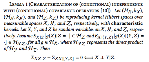
kernel-conditional-independence-test — **Lemma 1** (extracted from the paper)

where $\Sigma_{XX|Z} = \Sigma_{XX} - \Sigma_{XZ}\Sigma^{-1}_{ZZ}\Sigma_{ZX}$.

For all functions $g \in \mathcal{H_X}$ and $f \in \mathcal{H_Z}$, the cross-covariance operator $\Sigma_{ZX}: \mathcal{H_X} \longmapsto \mathcal{H_Z}$ of a random vector ($X, Z$) on $\mathcal{X} \times \mathcal{Z}$ defined in Fukumizu, Bach & Jordan (2004) is $$\langle f, \Sigma_{ZX}g \rangle_{\mathcal{H_Z}} = E_{XZ}[g(X)f(Z)] - E_X[g(X)]E_Z[f(Z)]$$

Additionally, the operator $\Sigma_{XX|Z}$ captures conditional variance of a random variable $X$ through $$\langle g, \Sigma_{XX|Z}g \rangle_{\mathcal{H_X}} = E_{Z}[Var_{X|Z}[g(X)|Z]]$$

Let $\ddot{Z} := [Y, Z]$. Similarly, we have $$\langle g, \Sigma_{XX|\ddot{Z}}g \rangle_{\mathcal{H_X}} = E_{\ddot{Z}}[Var_{X|\ddot{Z}}[g(X)|\ddot{Z}]]$$

2. Regression in RKHS

Given random variables $X, Z$ over measureable spaces $\mathcal{X}, \mathcal{Z}$, the authors exploit regression framework in RKHS to project $Z$ onto finite-dimensional $\mathcal{H_X}$, and encode the dependency by regressing $\phi_X(X)$ on $Z$ $$\phi_X(X) = F(Z) + U, \quad F: \mathcal{Z} \longmapsto \mathcal{H}_X \quad (1)$$ Consider the two regression models in RKHS $$\phi_X(X) = F_1(Z) + U_1, \quad \phi_X(X) = F_2(\ddot{Z}) + U_2 \quad (2)$$ From Lemma 1, we can derive the equality between the conditional variance operators as

eq4 — **Equation 4** (extracted from the paper)

$\phi_X(X)$ is a vector in infinite-dimensional space, and can be written as $ \phi_X(X) = [\phi_1(X), ..., \phi_i(X), ...]^T $. Since $\phi_X(X)$ is a feature map in $\mathcal{H}_X$, there exists a function $g \in \mathcal{H}_X$ such that $g = \phi_i(X)$. Thus, Equation 4 holds for any $\phi_i(X)$.

Furthermore, each component $\phi_i(X)$ and $\phi_j(X)$ is orthogonal, and $Cov(\phi_i(X), \phi_j(X))=0$ for $i \ne j$. Notice that $\phi_X(X)|Z$ is also a random vector with $ \phi_X(X)|Z = [\phi_1(X)|Z, ..., \phi_i(X)|Z, ...]^T $, the covariance matrix of $\mathsf{Var}[\phi_X(X)|Z]$ is a diagonal matrix in which each non-zero element corresponds to $\mathsf{Var}[\phi_i(X)]$ Thus, we can derive

eq3 — **Equation 3** (extracted from the paper)

Given $Z$, $Y$ gives no information to predict $X$. Graphically, if $Z$ is a parent of $X$ and $X$ and $Y$ are independent conditioning on $Z$, there should not be any arrow directly pointing to $X$ from $Y$. Thus, the first structural equation in (2) is a better fit. Here, causal learning can be viewed as a problem of model selection, and the task becomes how to construct a score function for selection regression model in RKHS.

The most straightforward test for goodness-of-fit is the maximum log-likelihood for the regression problem in (1). Unfortunately, we do not know the distribution of $\phi_X(X)$ since $\mathcal{X}$ is infinite-dimensional. The strategy is to reformulate the problem so that it is expressed only in kernel functions, which is tractable in finite space.

3. Formulation

For a particular observation $(x, z)$, we map $\phi_X(x)$ into the empirical feature map $k_X$ that is in $n$dimensional space $$ k_x = \left[ \begin{array}{cc|r} \langle k_X(x_1, x),\phi_X(x) \rangle_{\mathcal{H}_X} \\ ... \\ \langle k_X(x_n, x),\phi_X(x) \rangle_{\mathcal{H}_X} \end{array} \right] $$

According the reproducing property, $k_x$ has the same vector structure as $\phi_X(X)$ wherein each element is equivalent to a function $f_i(x)$ given by the linear combination. This means that regressing $k_X$ on $Z$ does not cause loss of information, that is the log-likelihood score reflects model compatibility while remains tractable.

We now turn our attention to the reformulated problem $$k_x = \tilde{F}(z) + \tilde{U} \quad (5) $$ Assuming Gaussian errors, we fit a kernel ridge regression on finite sample size (regression with $L2$ regularization) to estimate $$\tilde{\hat{F}}_Z(z) \approx \sum^{n}_{i=1} k_Z(z_i, z)c_i$$ where the coefficient matrix $c \in R^n$ can be found by solving $$\min \frac{1}{n}||Y-cK_Z||^{2}_{R^n} + \lambda c^T K_Z c \quad \lambda: \text{regularization parameter}$$ This gives $$\hat{c} = Y(K_Z + \lambda n I)^{-1}$$ The fitted function is $$\tilde{\hat{F}}_Z(z) = \hat{c}K_Z = \tilde{K_X}(K_Z + \lambda n I)^{-1}K_Z$$ The estimated covariance matrix is $$\hat{\Sigma} = \frac{1}{n}(\tilde{K}_X - \tilde{\hat{F}}_Z)(\tilde{K}_X - \tilde{\hat{F}}_Z)^T = n\lambda^2 \tilde{K}_X (\tilde{K}_Z + n\lambda I)^{-2}\tilde{K}_X $$

The maximal value of log-likelihood is represented as

**Maximum Value of Log-Likehood** (extracted from the paper)

From line 2 to line 3, $$\textsf{trace}\{(\tilde{K_X}-\hat{\tilde{W}}\Phi_Z)^T\hat{\Sigma}^{-1}(\tilde{K_X}-\hat{\tilde{W}}\Phi_Z)\} = \textsf{trace}\{\hat{\Sigma}^{-1}(\tilde{K_X}-\hat{\tilde{W}}\Phi_Z)^T(\tilde{K_X}-\hat{\tilde{W}}\Phi_Z)\}$$ $$=\textsf{trace}\{\hat{\Sigma}^{-1}(\tilde{K_X}-\tilde{\hat{F}}_Z)(\tilde{K_X}-\tilde{\hat{F}}_Z)^T\} = \textsf{trace}\{\hat{\Sigma}\hat{\Sigma}^{-1}\} = \textsf{trace}\{I\} = n$$

4. Score Functions

Maximizing the likelihood can cause over-fitting. Thus, the proposed score functions are Cross-Validation Log-Likelihood and Marginal Log-Likelihood.

4.1. CV Log-Likelihood

Given a dataset $D$ with $m$ variables $X_1, X_2, ..., X_m$, we split $D$ into a training set of size $n_1$ and a test set of size $n_0$, then repeat the procedure $Q$ times. Let $D^{(q)}_{1, i}$ and $D^{(q)}_{0, i}$ be the $q^{th}$ training set and the $q^{th}$ training set for variable $X_i$.

The score of DAG $\mathcal{G^h}$ is represented by $$S_{CV}(\mathcal{G^h}; D) = \sum^{m}_{i=1} S_{CV}(X_i, PA^{\mathcal{G^h}}_i)$$ $$S_{CV}(X_i, PA^{\mathcal{G^h}}_i) = \frac{1}{Q}\sum^{Q}_{q=1} l(\hat{\tilde{F^{(q)}_{i}}}|D^{(q)}_{0,i})$$ $X_i$ is the target variable and $PA^{\mathcal{G^h}}_{i}$ is the set of predictors in the regression function in Equation 5. The individual likelihood function is represented with kernel matrices as follow

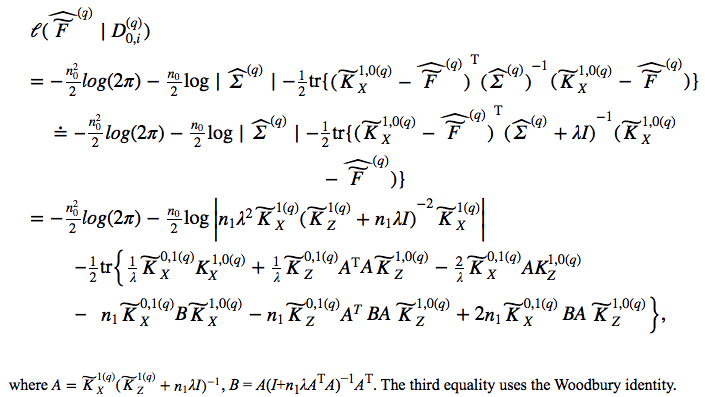
**CV Log-Likehood** (extracted from the paper)

The formula can be derived using matrix manipulation. Notice that line 2 approximates $\hat{\Sigma}^{(q)}$ by adding $\lambda$ to give rise to kernel functions. The paper also proposes removing the fitted values and using only $\widetilde{K_Z}$ to reduce overfitting. This is equivalent to regressing $k_X$ on the empty set. Please refer to the paper for more details.

4.2. Marginal Likelihood

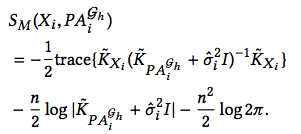
The marginal likelihood score is estimated as $$S_M(\mathcal{G^h};D) = \sum^{m}_{i=1} S_M(X_i, PA^{\mathcal{G^h}}_i)$$ with $S_M(X_i, PA^{\mathcal{G^h}}_i) = \mathsf{log} \ p(X_i|PA^{\mathcal{G^h}}_i, \hat{\sigma_i})$, and the noise variance $\hat{\sigma_i}$ is learned by maximizing marginal likelihood with gradient methods.

**Marginal Log-Likehood** (extracted from the paper)

Reliability

A score function must also satisfy Local Consistency and Score Equivalence.

Local Consistency

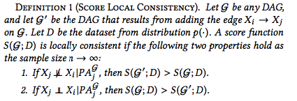
def1 — **Definition of Local Consistency** (extracted from the paper)

The score function is expected to give lower scores to models assigning with incorrect indendency constraints. It has been shown that under mild conditions, CV likelihood score is locally consistent according to Lemma 2.

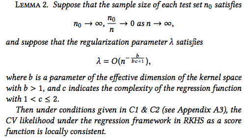
The model selected by CV likelihood has the same performance with the model selected by the optimal benchmark that is fitted on the entire sample. That is, CV likelihood score supports learning causal relations that hold in the true data generating distribution. This conclusion at the same time supports $K$-fold cross validation with reasonably large $K$.

Marginal likelihood score is also proven to yield local consistency according to Lemma 3.

The score can then be expressed in terms of Bayesian information criterion (BIC), plus a constant, in which BIC is locally consistent.

Score Equivalence

def2 — **Definition of Score Equivalence** (extracted from the paper)

On the other hand, the previous studies provide evidence that non-linear regression gives different scores to models in an equivalence class. Thus, neither CV or Marginal likelihood meet Score Equivalence.

However, the authors show that we can exploit local consistency and local score change to compare the reliability of any two DAGs. It is observed that the learned DAG with the same structure and orientation as the data generative distribution gives the highest scores. However, since there have not been any theoretical proof for this yet, we resort to the problem of searching the optimal Markov equivalence class.

In general, if conditions in Lemma 2 and Lemma 3 hold, the CV likelihood and Marginal likelihood, under RKHS regression framework, are guaranteed to find the Markov equivalence class that is closely consistent with the data generating distribution by using Greedy Equivalence Search algorithm (GES). Details can be found in Proposition 1 and Proposition 2.

Previous score-based methods

BIC, MDL : Estimating the Dimension of a Model
BGe : Learning Gaussian Networks
BDeu, BDe : Learning Bayesian networks: The combination of knowledge and statistical data.
BCCD : A Bayesian Approach to Constraint Based Causal Inference
Mixed BIC : Causal discovery from databases with discrete and continuous variables.
LiNGAM : LiNGAM: non-Gaussian methods for estimating causal structure
ICA-LiNGAM : A linear non-Gaussian acyclic model for causal discovery
Direct-LiNGAM : DirectLiNGAM: A direct method for learning a linear non-Gaussian structural equation model
ANM : Nonlinear causal discovery with additive noise models
CAM : CAM: Causal Additive Models, highdimensional order search and penalized regression
PNL : On the identifiability of the post-nonlinear causal model