Table of Contents
3.1. Putting It All Together
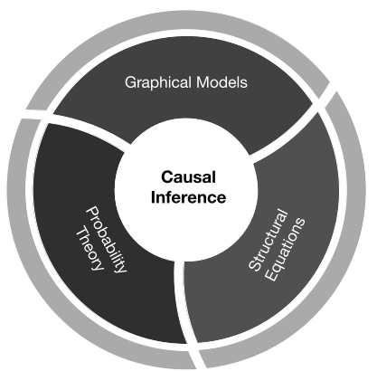
A causal model consists of a directed acyclic graph (DAG) over a set of random variables in which each variable is a node, and depedencies among variables are encoded in the edges. If there exists a directed edge pointing from a variable \(X\) to another variable \(Y\), we say \(X\) is a parent and a direct cause of \(Y\). A system of \(Y\) and all its parents form a causal mechanism for \(Y\). In such a mechanism, the value of \(Y\) is determined by the value of its parents through a stochastic function \(f\).

Chapter 1 introduces Bayesian Network as a toolkit to translate graphical language to probabilistic language. \(d-\)Separation is a test for graphical independency through the notion of blockage. According to Global Markov Assumption, the conditional independence yielded by a graph \(G\) licenses conditional independence with respect to the joint probability distribution \(P\), given that \(P\) adheres to the chain rule of Bayesian Network relative to \(G\).
The entire paradigm is buit upon a set of assumptions that render conditions under which causal inference frameworks can be applied. This means whenever given a dataset with probability distribution \(P\) and a causal graph \(G\), we must first test whether \(P\) and \(G\) are compatible.
We have also explained why correlation does not imply causation by examining the concept of Intervention. Statistical estimand \(P(Y|X)\) embedded in observational data is referred to associational distribution, while interventional distribution \(P(Y|do(X))\) is obtained through doing interventions on \(X\). The causal estimand \(P(Y|do(X))\) is what to be established for deriving the causal effect of \(X\) on \(Y\), while \(P(Y|X)\) is often a spurious signal.
Doing interventions is equivalent to conducting experiments by nature, specifically controlled randomized experiments. Part II will delineate why randomization is the key to causation, and the capacity of performing large-scale experiments efficiently is a valuable assset that tech companies should continue to exploit.
Intervention assumes the causal mechanisms are localized and independent. This means intervention on a variable only impacts its causal mechanism, leaving the rest of the system intact. The graph corresponding to intervention on a node is one constructed by deleting all arrows pointing into that node. Intervention on SCM is done by replacing the right-hand side of the structural equation with the value or distribution imposed by the intervention.
3.2. \(D.I.E\) Flowchart
3.2.1. Identification
Unfortunately, experimentation is not always feasible while observational data is massive. This is when Causal Inference wields its power. Chapter 2 presents fundamental techniques to identify causal effects from observational data with respect to a given causal model. The goal is to reduce causal estimands involving the \(do\) operator to statistical quantities to be computed from the data.
Non-parametric methods are generally preferable since they do not rely on any particular functional forms. Back-door criterion is the simplest solution to blocking confounding paths, which is often impractical due to unobserved confounders. Front-door criterion is proposed to address this limitation. \(Do-\)calculus is a set of inference rules to eliminate the \(do\) operator in a general setting. With a specified structural equation, Instrumental variable can be exploited for identification if such a variable can be found. Neverthles, one should note that not all causal estimands are identifiable.
3.2.2. Estimation
So far we have tackled Identification problems. Once settling with statistical estimands, the next task is estimation. Estimation can get challenging since it normally requires controlling for multiple variables. We may also come across heterogeneous treatment effects - effects varying by different groups of population. Part II explores estimation in more detail and Part IV zooms in on popular computer-assisted methods.
3.2.3. Discovery
Given a causal model, not only are we able to determine the causal relationships among variables of interest, but also to estimate the causal effects quantitatively from observational data. In several applications, especially high-dimensional settings, the causal graph remains unknown. Thus, we sometimes need to infer the causal graph from observational data. This is the problem of Causal Discovery or Structural Learning.
Causal learning algorithms from observational data can be broadly categorized into Constraint-based and Score-based approaches. The task, again, is to find the causal graph that aligns with the true data-generating process. Constraint-based methods uncover a set of causal graphs up to Markov equivalence class (groups of DAGs satisfying the same set of \(d-\)separation). They entail a series of conditional independence tests implemented independently with binary decisions of either accepting or rejecting the null hypothesis.
Meanwhile, score-based approach is more efficient in that it aims to evaluate the quality of a candidate causal graph according to a score function i.e., graphs with higher scores are better fits. Thus, the function must satisfy certain properties to be considered an appropriate goodness-of-fit test.
Both approaches generally assume Markov property (local at least), sufficiency (no unobserved confounders) and acyclicity (to be compatible with DAGs).
Causal discovery is a non-trivial task that fortunately can be automated. Not only do these libraries support learning causal structures but they also allow for modifications based on expertise knowledge. Curious readers are encouraged to go through the following materials
- Review of Causal Discovery Methods Based on Graphical Models (Glymour et al. 2019)
- Chapter 11 & 12 - Introduction to Causal Inference (Neal 2020)
In summary
It is impossible to identify causal relationships without the knowledge on the data generating process. We have seen that observational data do not tell a complete story, thus forcing us to make assumptions along the way to make the most use of it. This urges data practitioners to pay attention to the data collection process and product usage behavior.
$$Discovery \longrightarrow Identification \longrightarrow Estimation$$
3.3. Case Study: Job Training Partnership Act
The National JTPA Study was an initiative by the Department of Labor in the United States that aimed to measure the impact of a job training program on participants’ post-experimental earnings for 18 months. The study not only conducted randomized experiments but also collected observational data including data on non-participants.
Glynn and Kashin (2014) first evaluated the difference in average earnings between the experimental treatment group and the experimental control group, segregated by gender. The treatment group consisted of the individuals applying to the program and allowed to receive JTPA training services, while control group consists of randomly chosen individuals prevented from accessing the services.
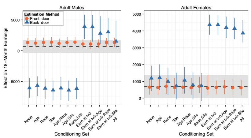
The results of observational causal analysis are benchmarked against the experimental results. Observational data was obtained by selecting program participants as well as non-participants, according to certain eligibility criteria, to fill out a survey inquiring about participation type and other background information. Glynn and Kashin compared the efficacy of back-door and front-door estimates, and empirically proved that the front-door criterion is a reliable alternative to randomized experiments in the presence of unobserved confounders.
What is interesting thing about the study is there were participants that signed up but did not show up in the treament group, i.e., non-compliers. Non-compliance is usually a nightmare in experimentation, but for such a causal analysis, it serves as a useful front-door criterion.
Figure 3.2 illustrates the causal graph for JTPA case study

The variables are summarized as follow
- \(Y:\) mean earnings in 18 months
- \(T:\) receving training (treatment) or not
- \(M:\) show up in training sessions (complier) or not
- \(X:\) other covariates such as demographics, social program participation, training and education histories
- \(U:\) unobserved or immeasurable confounding variables such as motivation
Blocking the back-door path opened up by \(X\), the back-door estimate is $$P^{bd}(y|do(T)=t) = \sum_x P(y|x,t)P(x) \quad (1)$$
On the other hand, we can also use \(M\) as a front-door criterion. However, conditioning on \(M\) alone opens up the back-door path \(T \leftarrow X \rightarrow Y\). We therefore must condition on \(X\) as well. $$P^{fd}(y|do(T)=t) = \sum_x \sum_m P(m|t,x)\sum_{t'} P(y|t', m, x)P(t')P(x) \quad (2)$$
Both estimates are biased, since there exists an unblocked back-door path created by \(U\). However, Glynn and Kashin demonstrated that, in case the effect of \(U\) on \(M\) is is sufficiently small or due to randomness (for example, bad weather made some participants less motivated to show up), the front-door estimate approximates the experimental benchmarks. Meanwhile, back-door adjustment turned out to give a poor estimate, and such covariates were shown not sufficient conditioning sets to mitigate the biases caused by unobserved confounders.

Causal Effect in the Treated
In the case study, the authors did not measure the standard causal effect as indicated in \((1)\) and \((2)\). In many social applications, the causal effect in the treated is of interest. The technique effectively assumes that treatment assignment has no effect if treatment is not received. Thus, we only examine the participants who signed up for the training i.e., \(T=1\). Denoting this group as \(T_1\), we extend \((1)\) and \((2)\) as follows
Back-door Adjustment for the Treated
$$P^{bd}(y|do(T)=t, T_1) = \sum_x P(y|x,t)P(x|T_1)$$ An important note is the quantity \(P(y|do(T)=0, T_1)\) measures the effect on \(Y\) had the treated not been treated, which contradicts the reality in which all individuals in \(T_1\) were actually treated. \(P(y|do(T)=0, T_1)\) is thus said to be counterfactual and can be estimated as $$P^{bd}(y|do(T)=0, T_1) = \sum_x P(y|x,T=0)P(x|T=1)$$ And the "factual" interventional distribution from \(do(T)=1\) is $$P^{bd}(y|do(T)=1, T_1) = P(y|T_1) = P(y|T=1)$$
Front-door Adjustment for the Treated
$$P^{fd}(y|do(T)=t, T_1) = \sum_x \sum_m P(m|t,x)\sum_{t'} P(y|t', m, x)P(t'|T_1)P(x|T_1)$$ Because \(P(t=1|T_1) = 1\) and \(P(t=1|T_1) = 0\), the expression becomes $$P^{fd}(y|do(T)=t, T_1) = \sum_x \sum_m P(m|t,x) P(y|T_1, m, x)P(x|T_1)$$ Similarly, we have $$P^{fd}(y|do(T)=1, T_1) = P(y|T_1) = P(y|T=1) $$
Note that \(P(M=0|T=0, x)=1\) and \(P(M=1|T=0, x)=0\) i.e., the non-treated never shows up. The counterfactual distribution is $$P^{fd}(y|do(T)=0, T_1) = \sum_x P(y|T_1, M=0, x)P(x|T_1) = \sum_x P(y|T=1, M=0, x)P(x|T=1) $$
Again, the quantities on the right-hand side of these equations can be easily derived out of observational data.
3.4. Pearl's Causal Reasoning Hierarchy
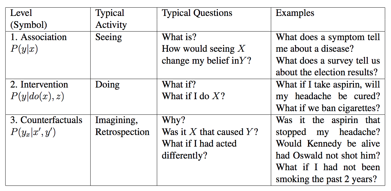
The JTPA case study exposes us to the concept of Counterfactuals. We have also seen that although the counterfactual terms describe non-existent or imaginary events, it is sometimes possible to estimate them from observational data. An important application of Counterfactuals is Mediation Analysis, and we will see more details of these concepts in the next chapter.
Counterfactual fits in a bigger picture of Pearl's Causal Ladder, which nicely summarizes what Causality is in a nutshell. To reason causally is to find the answers to the following queries

